Comparing utilisation distributions

Once you have several UDs — for different individuals, different seasons, or different behavioural contexts (see vignette("UD_bursted_uds", package = "move2utils")) — the next question is usually how similar they are. This vignette covers the three comparison operations: stacking on a common grid, computing an overlap metric, and computing Earth-mover’s distance (EMD).

Stacking on a common grid

Every pairwise UD metric depends on the two UDs having identical extents and cell geometry. mt_dbbmm_ud() and mt_dbgb_ud() enforce this automatically on multi-track input. The only situation where you need to intervene manually is when the UDs come from separate dispatches (e.g. two datasets loaded at different times).

This is how you can get a stack with each layer renormalised to sum to 1:

## Given a list of UDs (or a multi-layer SpatRaster) on a common grid:
uds_list <- list(day = ud_day, night = ud_night)                # or split

stk <- terra::rast(uds_list)                                     # stack
stk <- stk / terra::global(stk, "sum", na.rm = TRUE)[, 1]        # renormalise
names(stk) <- names(uds_list)

The global(..., "sum") divisor is a per-layer scalar, so the division broadcasts correctly and every output layer sums to 1 . If you built the UDs with mt_dbbmm_ud() or mt_dbgb_ud()’s multi-track dispatch, or with the composite-track_id idiom from vignette("UD_bursted_uds", package = "move2utils"), the output is already on a common grid and already per-layer normalised — you do not need the renormalisation step.

library(move2)
library(dplyr)
library(sf)
library(terra)
library(move2utils)

fishers <- mt_read(mt_example())
fishers <- fishers[!st_is_empty(fishers), ]

two <- filter_track_data(fishers, .track_id = c("F3", "M3"))
## keep each individual to its first 500 fixes for a fast build
two <- two |>
  dplyr::group_by(mt_track_id(two)) |>
  dplyr::slice_head(n = 500) |>
  dplyr::ungroup()
two_p <- st_transform(two, mt_aeqd_crs(two))

stk <- mt_dbbmm_ud(
  two_p,
  location_error = 25,
  window_size    = 31,
  margin         = 11,
  raster         = 100,
  ext            = 1.25
)
names(stk)
#> [1] "F3" "M3"

stk and vud are both a two-layer SpatRaster; the layers share grid and CRS.

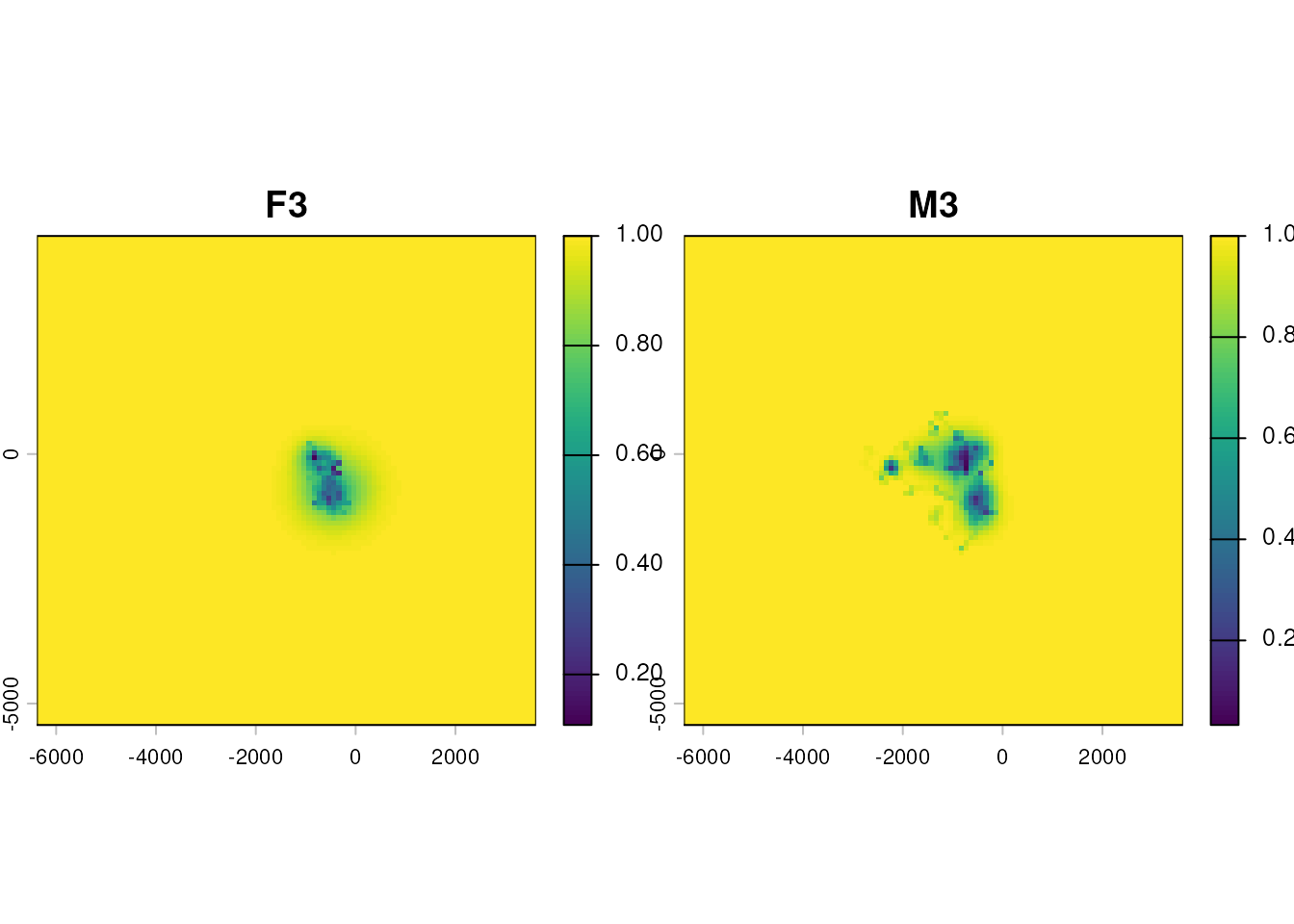
Volume UD

Most comparison operations work more cleanly on cumulative-volume UDs than on raw probability densities. The transform orders cells by probability density and replaces each value by the cumulative sum — so cell v = 0.5 means “this cell is inside the 50 %-volume contour, together with all denser cells”. ud_volume() applies the transform; it accepts a multi-layer SpatRaster and acts layer-wise.

vstk <- ud_volume(stk)
names(vstk)
#> [1] "F3" "M3"
terra::plot(vstk)

Overlap metrics

Volume of intersection

The fraction of the smaller UD that falls inside the larger UD’s 50 % (or 95 %, or p) volume contour is a common “core-area overlap” summary.

in_core <- function(vud_a, vud_b, p = 0.5) {
  mask_a <- vud_a <= p
  mask_b <- vud_b <= p
  sum(terra::values(mask_a & mask_b), na.rm = TRUE) /
    sum(terra::values(mask_a | mask_b), na.rm = TRUE)
}

in_core(vstk[[1]], vstk[[2]], p = 0.50)   # 50% core overlap
#> [1] 0.2461538
in_core(vstk[[1]], vstk[[2]], p = 0.95)   # 95% use overlap
#> [1] 0.5148515

Bhattacharyya affinity

A density-level overlap on the raw probability UDs; bounded in [0, 1], 1 meaning identical distributions.

bhatt <- function(p, q) {
  p <- terra::values(p); q <- terra::values(q)
  sum(sqrt(p * q), na.rm = TRUE)
}
bhatt(stk[[1]], stk[[2]])
#> [1] 0.7916157

Because both UDs already sum to 1 on the same grid, the returned value is exactly the Bhattacharyya affinity used in the home-range literature (e.g. Fieberg & Kochanny 2005).

A visual: where the two UDs agree and disagree

diff_ud <- stk[[1]] - stk[[2]]
terra::plot(diff_ud,
            main = "F3 UD - M3 UD",
            col = hcl.colors(100, "Blue-Red 3"))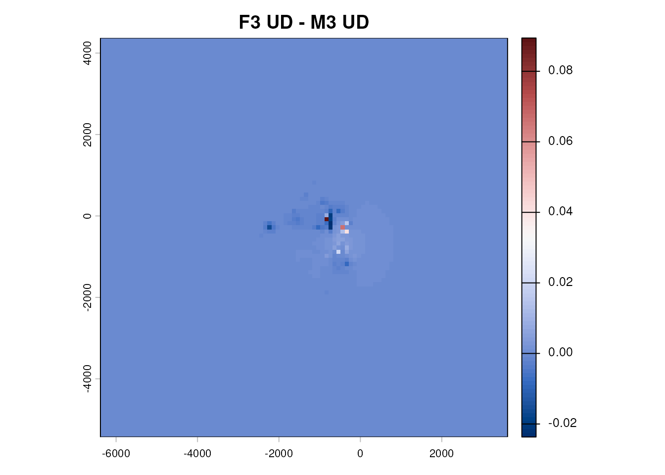

Positive cells belong more to F3; negative to M3. Neutral grey indicates the shared core.

Earth-mover’s distance (EMD)

EMD is the minimum-cost work to transport probability mass between two UDs; it decreases smoothly as the two UDs drift into coincidence. emd() computes pairwise EMDs over a stack of UDs and returns a stats::dist object.

d <- emd(stk)
d
#>          F3
#> M3 528.0358

By default emd() uses Sinkhorn entropic regularisation (Cuturi 2013). On a 5-UD fisher stack the default call completes in well under a minute. A mask_quantile = 0.999 pre-mask (via ud_volume()) drops cells outside the 99.9 % volume contour — typically > 95 % of cells on well-supported UDs — before transport, and is the single biggest practical speed-up.

For validation you can switch to the exact LP solver (requires the emdist package):

d_exact <- emd(stk, method = "exact")

## relative difference between Sinkhorn and exact, typically sub-1%
max(abs(as.vector(d) - as.vector(d_exact)) / as.vector(d_exact))

Unprojected (lon/lat) UDs and a hard distance cutoff

emd() defaults to Euclidean distance between cell centroids, which is the right ground metric on projected UDs. If your UDs are on a longitude/latitude grid (e.g. straight from terra::rast() without mt_aeqd_crs()), pass gc = TRUE to use Haversine great-circle distances instead — emd() warns when input is on a longlat CRS and gc = FALSE. The threshold argument (in map units when gc = FALSE, metres when gc = TRUE) clips the cost matrix at a maximum transport distance, reproducing the EMD-hat variant exposed by move::emd(). Both gc and threshold are currently honoured by method = "sinkhorn" only; method = "exact" is restricted to Euclidean, unclipped costs through emdist::emd().

Tuning `reg` and `mask_quantile`

What for	`reg`	`mask_quantile`	Expected behaviour
Default (balanced)	0.05	0.999	Fast; within 0.1 % of exact
Fastest (interactive)	0.1	0.95	Very fast; within 1 %
Highest fidelity	0.01	0.9999	Slow; near-exact
Exact	—	0.999	Use `method = "exact"`

On irregularly supported or multi-modal UDs, consider raising mask_quantile slightly so that secondary modes are not truncated.

Pairwise comparison across a UD stack

Any metric that takes two UDs generalises to a distance matrix on a stack. For a small number of UDs, a nested sapply is fine:

ud_list <- lapply(seq_len(terra::nlyr(stk)), function(i) stk[[i]])
nm      <- names(stk)

mat <- outer(seq_along(ud_list), seq_along(ud_list),
             Vectorize(function(i, j) bhatt(ud_list[[i]], ud_list[[j]])))
dimnames(mat) <- list(nm, nm)
mat

For larger stacks the emdist EMD is the bottleneck (it is super-linear in the number of non-zero cells), so downsample the grid or mask to a tight contour first.