Diagnosing an mt_clean_track run

mt_clean_track() returns a result, but did it work? mt_diagnose_clean_track() is the post-run health check — six panels analogous to plot.lm() for a GLM, each addressing a distinct failure mode and pointing at a specific remedy when something looks off. It does not re-run the detectors; it reads the flag columns and the underlying step speeds, and renders one figure that lets you eyeball whether the run was healthy.

library(move2)
library(sf)
library(move2utils)

A run that needs attention — Pettstadt1, a juvenile white stork

Pettstadt1 is a juvenile white stork (~3 kg) with 48k GPS fixes spanning two summers and one autumn migration. We clean it and then run the diagnostic.

pet <- mt_read(system.file("extdata/Pettstadt1-14053.csv.gz",
                              package = "move2utils"))
pet <- pet[!st_is_empty(pet), ]
pet <- mt_filter_unique(pet, criterion = "first")
pet <- dplyr::arrange(pet, mt_track_id(pet), mt_time(pet))
res_pet <- mt_clean_track(pet, mass = 3, mode = "flying",
                            plot = FALSE, remove = FALSE,
                            silent = TRUE,
                            max_flag_fraction = 0.5)
cat(sprintf("Pettstadt1: %d / %d flagged (%.2f%%)\n",
            sum(res_pet$is_outlier), nrow(res_pet),
            100 * mean(res_pet$is_outlier)))
#> Pettstadt1: 4133 / 48239 flagged (8.57%)

The flag fraction is high — likely beyond what genuine GPS errors would produce on a stork. Time to ask the diagnostic what happened.

diag <- mt_diagnose_clean_track(res_pet)
#> === mt_diagnose_clean_track: concerns flagged ===
#> Panel 1: 3 substantive modes detected at 0.01, 0.95, 8.51 m/s -- bimodal behaviour. The per-fix detectors threshold against a single distribution; consider state-conditional analysis or filtering to one mode before cleaning.
#> Panel 2: sustained band of elevated flag rate detected -- this is the migration-over-flagging signature. Consider filtering that window or running it through state-conditional analysis.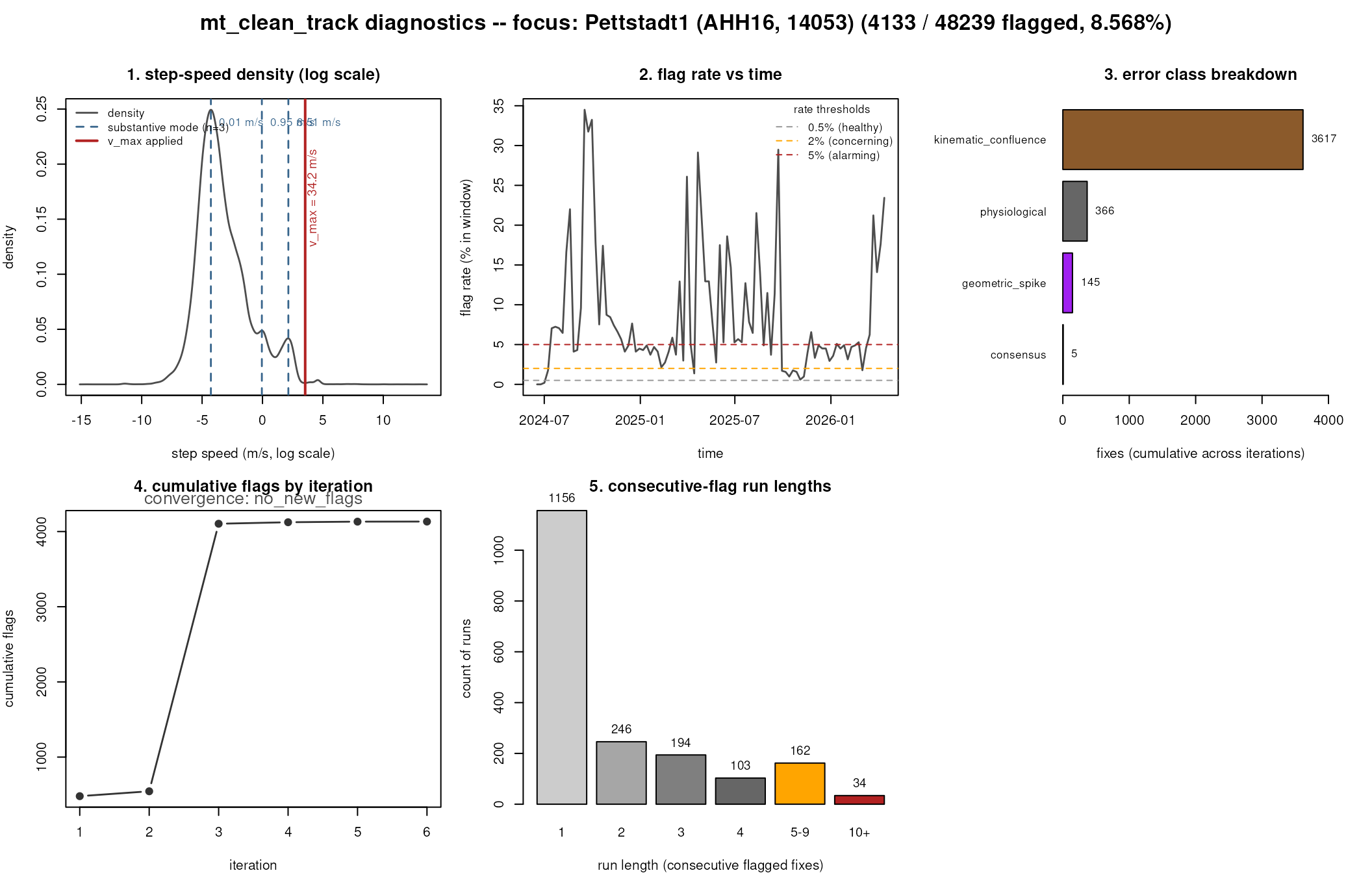

The function prints the concerns it found and renders six panels.

Reading the panels

Panel 1 — log-speed density with detected modes. The grey curve is the distribution of step speeds on log scale; the blue dashed lines mark the substantive modes the package detected (basin holds at least 2 % of fixes and peak density ≥ 5 % of the global peak). The red line is the v_max that was used. Healthy: a single dominant mode with a sparse upper tail. What you’ll see on Pettstadt1: two or three modes — sleeping/perched at the lower end, and a flight mode further right. Multiple substantive modes is the bimodal-behaviour signature: the per-fix detectors threshold against a single distribution, so one mode’s fixes can land in the tail of the other and look like outliers.

Panel 2 — flag rate vs time. Rolling 7-day flag rate over the timeline. Healthy tracks read flat, near 0 %, with isolated narrow spikes only where the bird had a real GPS noise event. What you’ll see on Pettstadt1: a sustained band of elevated flag rate during the autumn migration months. Sustained ≠ outliers — sustained ≈ “the bird was doing something the detector wasn’t calibrated for”.

Panel 3 — per-detector activity. Counts of fixes flagged by each detector combination, summed across all iterations. With the class-aware default flag rule, the headline categories are consensus (≥3 of 4 detectors agree), geometric_spike (bridge AND detour), state_anomaly ((bridge|detour) AND speed), and kinematic_confluence ((bridge|detour) AND prob); these interpretations are encoded in the error_class column. Single- detector bars (bridge-only / detour-only / prob-only / speed-only) are fixes one detector flagged but the class rules did not promote to a flag — useful information about which detector is firing noisily on this track. On Pettstadt1 expect bridge+prob to dominate (kinematic_confluence): bridge says “fix sits far from a straight- line interpolation between neighbours” and prob says “this fix’s joint speed/turn signature lies in the tail of the empirical distribution”. Both are correct relative to the resting baseline, both are wrong as errors during migration.

Panel 4 — cumulative flagging by iteration. Rapid plateau in 2–4 iterations is healthy — the iteration loop converges on a stable flag set. Linear growth without plateau, especially if the run hits the flag_fraction_exceeded abort, is the non-converging signature: each iteration peels off another batch as the active set keeps shifting. There is no fixed point because the underlying mismatch (bimodal distribution against single-distribution thresholds) cannot be resolved by iterating.

Panel 5 — consecutive-flag run lengths. Healthy: tall length-1 bar, short tail. The orange and red bins (“5–9”, “10+”) count runs of consecutively flagged fixes — long runs are not what discrete GPS errors look like; they are what happens when the bird flies through a region the detector treats as “anomalous” for hours at a time.

The diagnostic notes printed by mt_diagnose_clean_track() summarise these patterns in plain language and point at the remedy.

A clean run for contrast — CPF_B (synthetic, no truth outliers)

The bundled CPF_B track is documented as clean (no injected outliers). A healthy run + diagnostic should look very different from Pettstadt1.

syn <- mt_read(system.file("extdata/synthetic_tracks.csv.gz",
                             package = "move2utils"))
syn <- syn[!st_is_empty(syn), ]
m_B <- syn[mt_track_id(syn) == "CPF_B", ]
res_B <- mt_clean_track(m_B, plot = FALSE, remove = FALSE, silent = TRUE)
cat(sprintf("CPF_B: %d / %d flagged (%.4f%%)\n",
            sum(res_B$is_outlier), nrow(res_B),
            100 * mean(res_B$is_outlier)))
#> CPF_B: 0 / 3537 flagged (0.0000%)
mt_diagnose_clean_track(res_B)
#> === mt_diagnose_clean_track: no concerns flagged. ===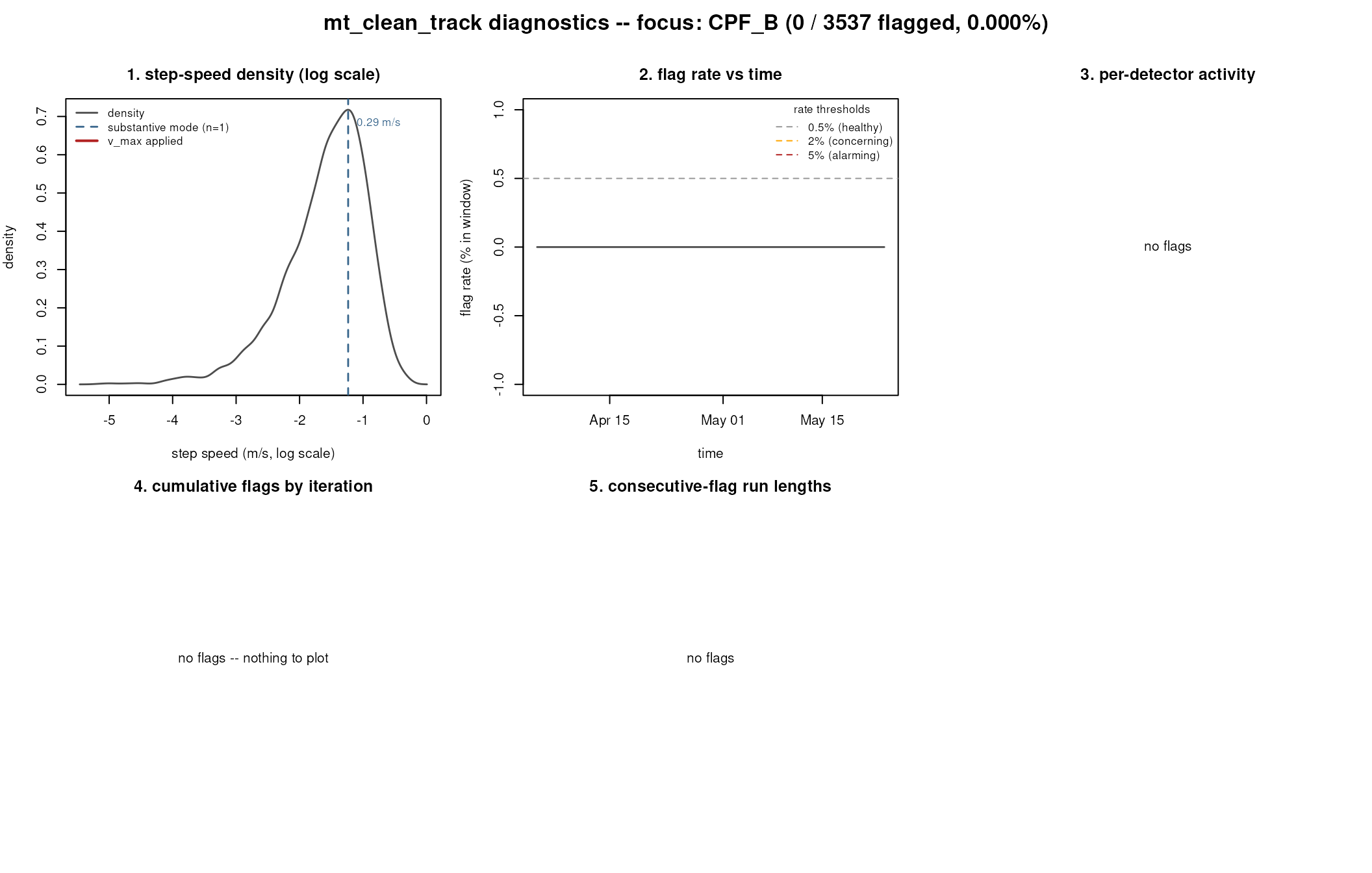

What you see: Panel 1 has a single dominant mode, Panel 2 is flat, Panel 3 has zero or almost-zero bars, Panel 4 plateaus at iteration 1, Panel 5 shows mostly run length 1 (or no flags at all). The diagnostic prints “no concerns flagged” — the run was healthy.

A multi-individual study

When you pass a multi-track result, panels 1–5 focus on the individual with the highest flag rate by default, and panel 6 shows a per- individual dotplot for at-a-glance triage of which animals to inspect next. Pass individual = "..." to focus a specific track.

res_multi <- mt_clean_track(study, mass = my_mass_named, mode = "flying",
                              compact = TRUE, plot = FALSE, remove = FALSE)

## Default focus = highest-flag-rate individual
mt_diagnose_clean_track(res_multi)

## Or focus on a specific bird
mt_diagnose_clean_track(res_multi, individual = "Benjamin 7206 E0706")

A decision tree for what to do next

Diagnostic signature	Likely cause	Remedy
Multiple substantive modes (Panel 1)	Bimodal behaviour (rest + flight)	State-conditional analysis (see `vignette("OUTLIER_3_state_conditional", package = "move2utils")`); or filter to one state
Sustained band of elevated flag rate (Panel 2)	Migration period being mistaken	Filter the migration window or run it through state-conditional analysis
Single-detector bars dominate (Panel 3)	One detector noisy on this track; class rules did not promote	Inspect those flags manually; consider raising that detector’s threshold
Iteration not plateauing (Panel 4)	Self-reinforcing flagging	Check Panel 1; supply a hard `v_max`; or use state-conditional analysis
Long-run tail without `error_class = "block"` (Panel 5)	Sustained behavioural state	Same as Panel 2 / 4
Several individuals at >2 % (Panel 6, multi)	Cohort heterogeneity	Triage list; run state-conditional or hard-cap path on the >5 % individuals

When several panels light up together with the same root cause — bimodal distribution + sustained migration band + non-converging iteration + heavy run-length tail — the answer is almost always state-conditional analysis.

What the diagnostic does not do

It does not re-run the per-fix detectors. The bridge-η and joint- probability distributions, which would let you see whether the score threshold landed in a real density valley or cut through a continuum, are not currently part of the suite — adding a “recompute = TRUE” panel for those is a planned extension.

It also assumes a single behavioural-state threshold was applied. Tracks where you have already segmented by state and run mt_clean_track per segment will read “healthy” on every panel because each segment IS unimodal.