Dynamic Brownian bridge UDs (dBBMM)

Here we present a workflow for the calculation of dynamic Brownian bridge movement models (dBBMM) and UDs. We have updated the dBBMM related functions from the move package to use move2, sf and terra, and in the process also improved the algorithm which is now much faster. If you have migrated from move, the translation is:

legacy `move`	`move2utils`
`spTransform(x, center = TRUE)`	`sf::st_transform(x, move2::mt_aeqd_crs(x))`
`brownian.motion.variance.dyn()`	`mt_dbbmm_variance()`
`brownian.bridge.dyn()`	`mt_dbbmm_ud()` (or the two-step variance → UD)
`getMotionVariance()`	`mt_motion_variance()`
`getVolumeUD()`	`ud_volume()` (or the inline recipe shown below)

There are two main functions in the workflow: mt_dbbmm_variance() estimates a dynamic Brownian-motion variance per location, and mt_dbbmm_ud() rasterises the bridge-weighted UD on a common grid.

Load and project a track

library(move2)
library(sf)
library(dplyr)
library(terra)
library(move2utils)

## get move2 example data set: fishers GPS data
fishers <- mt_read(mt_example())
fishers <- fishers[!st_is_empty(fishers), ]

## Leroy (M1); keep the first few hundred
## locations so the vignette builds quickly
leroy <- filter_track_data(fishers, .track_id = "M1")
leroy <- slice(leroy,1:500)

## dBBMM needs a projected CRS; an AEQD projection centred on the
## track is convenient and keeps units in metres
leroy_p <- st_transform(leroy, mt_aeqd_crs(leroy))
nrow(leroy_p)
#> [1] 500

Fit a dBBMM

The two-step workflow separates variance estimation from UD rasterisation so that you can reuse the variance object when tuning the grid. Pass location_error in map units (metres here); window size and margin control the sliding estimator (see ?mt_dbbmm_variance). Note that in most cases different values of window size and the margin do not have a great effect on the results.

var_obj <- mt_dbbmm_variance(
  leroy_p,
  location_error = 20,
  window_size    = 31,
  margin         = 11
)

## a numeric vector of per-location variances (NA at track margins)
head(mt_motion_variance(var_obj))
#> [1] NA NA NA NA NA NA

Rasterise the UD. There are two options, either set the cell size of the raster, e.g. raster = 100 requests a 100 m cell size; or pass a pre-made SpatRaster when you need UDs from different tracks on a shared grid.

ud <- mt_dbbmm_ud(var_obj, location_error = 20, raster = 100)
#> Computational size: 3.2e+08

terra::plot(ud, main = "dBBMM utilisation distribution")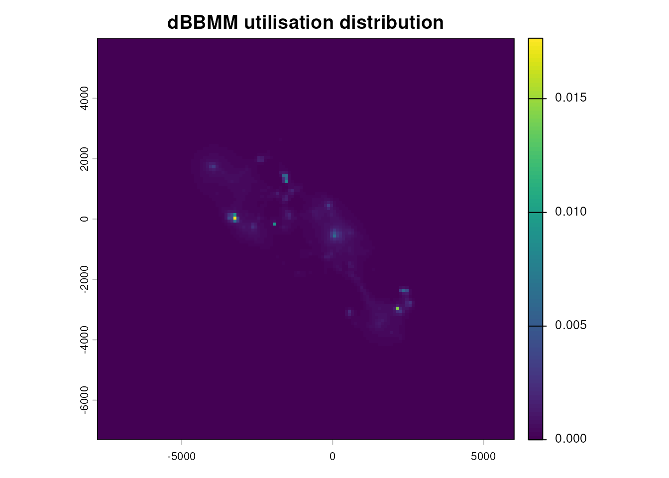

The single-step shortcut mt_dbbmm_ud(leroy_p, location_error = 20) fits the variance internally — convenient when you do not need the variance object itself.

The sum of all pixels of the dBBMM UD raster sum up to 1. Plotting the result provides limited visual information, as the values correspond to the probability the animal was present in a given pixel during the observed period. These results can be used to estimate probability of the animal being present in a certain area during the tracking period (see ‘Cumulative-volume UD’ section), or to calculate the probability of the animal being present in a certain environment during the tracking period by overlaying the resulting raster over a categorical raster (e.g. of land cover) and summing up the dBBMM pixel values that fall within each category.

Cumulative-volume UD and isopleths

ud_volume() converts a UD into cumulative-probability space, which represents the minimum area in which an animal has some specified probability of being located. (This is the move2 analogue of move::getVolumeUD().)

vud <- ud_volume(ud)
terra::plot(vud, main = "Cumulative volume UD")
terra::contour(vud, levels = c(0.5, 0.95), add = TRUE,
               lty = c(2, 1), lwd = c(0.5, 0.5))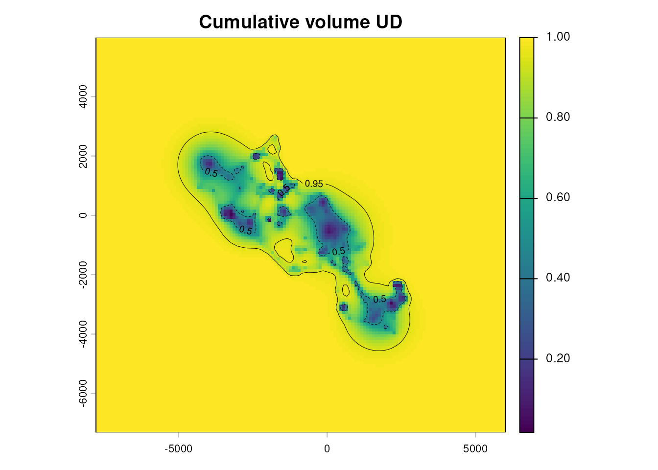

Solid 50 % and 95 % masks are simple logical operations on the volume UD:

ud50 <- vud <= 0.50
ud95 <- vud <= 0.95

par(mfrow = c(1, 2))
terra::plot(ud95, main = "95% area", col = c("grey90", "steelblue"))
terra::plot(ud50, main = "50% area", col = c("grey90", "firebrick"))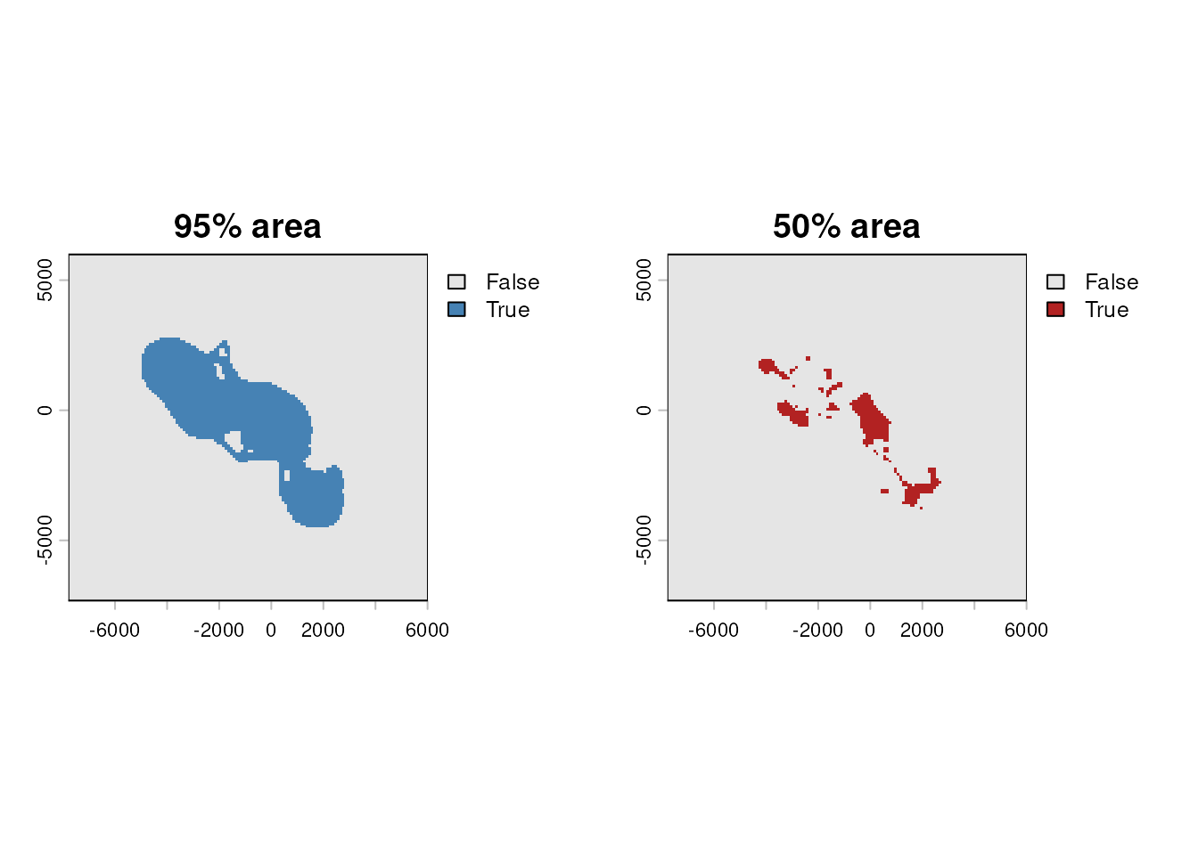

If you need the isopleth as a vector (line or polygon), terra’s own as.contour() returns a SpatVector that coerces cleanly to sf:

iso95 <- terra::as.contour(vud, levels = 0.95) |>
  sf::st_as_sf()

Handling gaps and the time-step pitfall

Choose a sensible `time_step`

mt_dbbmm_ud() integrates the Brownian bridge along each segment. The step defaults to 1/15 of the smallest time lag in the track, which keeps the quadrature stable for short segments. Inspect your time lags before fitting so you know what you’re working with:

lags <- as.numeric(mt_time_lags(leroy_p, units = "min"))
summary(lags)
#>    Min. 1st Qu.  Median    Mean 3rd Qu.    Max.     NAs 
#>   13.27   14.73   15.05   33.94   15.49  976.70       1

If you have a track with a median lag much larger than the minimum, and very few short lags, you can override time_step = median(lags)/15 to speed things up; but keep the smallest lag governing the step when short segments carry real information about rapid movement.

Do not bridge across long gaps

A missing satellite pass leaves a long time lag between otherwise adjacent fixes. Integrating the bridge across that gap smears probability across regions the animal never visited. The fix is to mark those locations as “not of interest” in the variance object before rasterising; the UD integration will skip them.

We construct an artificial gap by removing a block of fixes, and compare the UD with and without the mask:

## introduce a synthetic 6-hour gap
keep <- setdiff(seq_len(nrow(leroy_p)), 200:260)
leroy_gap <- leroy_p[keep, ]

var_gap <- mt_dbbmm_variance(
  leroy_gap, location_error = 20,
  window_size = 31, margin = 11
)

## the UD with no gap masking — probability bleeds across the gap
ud_bleed <- mt_dbbmm_ud(var_gap, location_error = 20, raster = 100,
                         verbose = FALSE)

## mask out locations whose following segment exceeds 300 minutes
lag_gap <- as.numeric(mt_time_lags(leroy_gap, units = "min"))
var_gap$interest[which(lag_gap > 300)] <- FALSE

ud_masked <- mt_dbbmm_ud(var_gap, location_error = 20, raster = 100,
                          verbose = FALSE)

## for better visualization plotting the cumulative volume UD
par(mfrow = c(1, 2))
terra::plot(ud_volume(ud_bleed),  main = "unmasked: bleeds across gap")
terra::plot(ud_volume(ud_masked), main = "masked: clean")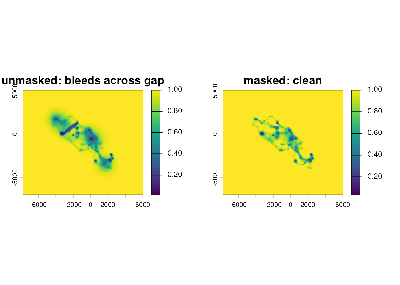

The difference is usually visible as a low-density ribbon connecting the two sub-tracks; masking removes it.

Multi-individual UDs on a common grid

Both mt_dbbmm_variance() and mt_dbbmm_ud() dispatch on multi-track move2 objects: they return a named list of variance objects and a multi-layer SpatRaster respectively, all on a grid computed from the combined extent so that layers are directly comparable.

three <- fishers[mt_track_id(fishers) %in% c("F1", "F2", "M1"), ]
three_p <- st_transform(three, mt_aeqd_crs(three))

stk <- mt_dbbmm_ud(three_p, location_error = 25,
                    window_size = 31, margin = 11)
names(stk)
terra::plot(stk)

Persistence

The package does not ship its own IO helpers — the sf and terra ecosystems already provide every format the legacy move vignette covered (shapefile, GeoTIFF, GeoPackage, KML, CSV).

saveRDS(var_obj, "leroy_dbbmm_variance.rds")
terra::writeRaster(ud, "leroy_ud.tif", overwrite = TRUE)
sf::st_write(leroy, "leroy.gpkg", delete_layer = TRUE)