Producing one UD per behavioural state (day/night, season, etc.)

Sometimes you don’t want one UD per animal — you want one UD per context: this bird’s daytime UD vs. its nighttime UD, this animal’s summer range vs. its winter range, this seal’s foraging UD vs. its haul-out UD. The pattern: you have a category that varies within one track, and you want a separate UD for each category, stacked together on a common grid so they’re directly comparable.

This vignette shows two ways to do that with mt_dbbmm_ud() and mt_dbgb_ud(). The first uses the existing multi-track dispatch (by attaching the context to the track ID); the second uses split() + lapply when each context needs different settings.

(If you used the legacy move package’s MoveBurst class, this is the move2 equivalent. move2 deliberately doesn’t reproduce MoveBurst — context belongs on the tibble as a column, and the per-context workflow is expressible directly with dplyr and the package’s normal multi-track dispatch. The result is the same kind of stacked UD output you’d get from DBBMMBurstStack.)

Two idioms

A. Composite `track_id`

Make the context part of the track identifier. The existing multi-track dispatch of mt_dbbmm_ud() / mt_dbgb_ud() then does exactly what MoveBurst used to do: one UD per composite label, stacked on a common grid.

B. `split()` and iterate

Keep the original track_id. Split the object into a list of sub-tracks, one per context, and lapply the UD function. Needed when contexts require their own grids or settings.

A is the default; B is the fallback.

Setting the scene

library(move2)
library(dplyr)
library(sf)
library(terra)
library(move2utils)

fishers <- mt_read(mt_example())
fishers <- fishers[!st_is_empty(fishers), ]

## three individuals with enough data for a reasonable per-burst UD
ids <- c("F1", "F2", "M1")
focal <- filter_track_data(fishers, .track_id = ids)
focal <- focal |> dplyr::group_by(mt_track_id(focal)) |> slice(1:500) |> ungroup()
focal_p <- st_transform(focal, mt_aeqd_crs(focal))

Attaching a per-location context column

The simplest contexts are per-location (length n): derived from the timestamp (hour-of-day, season), from an environmental annotation (habitat class), or from a downstream classifier (HMM state). Attach them as columns.

focal_p <- focal_p |>
  dplyr::mutate(
    hour       = as.integer(format(mt_time(focal_p), "%H")),
    day_night  = factor(
      dplyr::if_else(hour >= 6 & hour < 18, "day", "night"),
      levels = c("day", "night")
    )
  )
table(focal_p$day_night, mt_track_id(focal_p))
#>        
#>          F1  F2  F3  M1  M2  M3  M4  M5
#>   day   248 181   0 239   0   0   0   0
#>   night 252 319   0 261   0   0   0   0

For per-segment contexts (length n-1), align them to the starting location of each segment and pad the final location with NA or with the last segment’s label — whichever matches your intent.

Idiom A — composite `track_id`

Build a composite label and set it as the track identifier. Existing multi-track dispatch handles the rest.

focal_burst <- focal_p |>
  dplyr::mutate(
    burst_id = paste(mt_track_id(focal_p), day_night, sep = "__")
  )
focal_burst <- mt_set_track_id(focal_burst, "burst_id")

table(mt_track_id(focal_burst))
#> 
#>   F1__day F1__night   F2__day F2__night   M1__day M1__night 
#>       248       252       181       319       239       261

A dBBMM UD per `(individual, day/night)` pair

mt_dbbmm_variance() accepts a multi-track move2 object and returns a named list of variance objects. mt_dbbmm_ud() on that list rasters each UD on a common grid computed from the combined extent, so the layers are directly comparable.

var_list <- mt_dbbmm_variance(
  focal_burst,
  location_error = 25,
  window_size    = 31,
  margin         = 11
)
length(var_list)
#> [1] 6
names(var_list)
#> [1] "F1__night" "F1__day"   "F2__day"   "F2__night" "M1__day"   "M1__night"

stk <- mt_dbbmm_ud(var_list, location_error = 25, raster = 100,
                    ext = 0.85, verbose = FALSE)
names(stk)
#> [1] "F1__night" "F1__day"   "F2__day"   "F2__night" "M1__day"   "M1__night"
vud <- ud_volume(stk)
terra::plot(vud)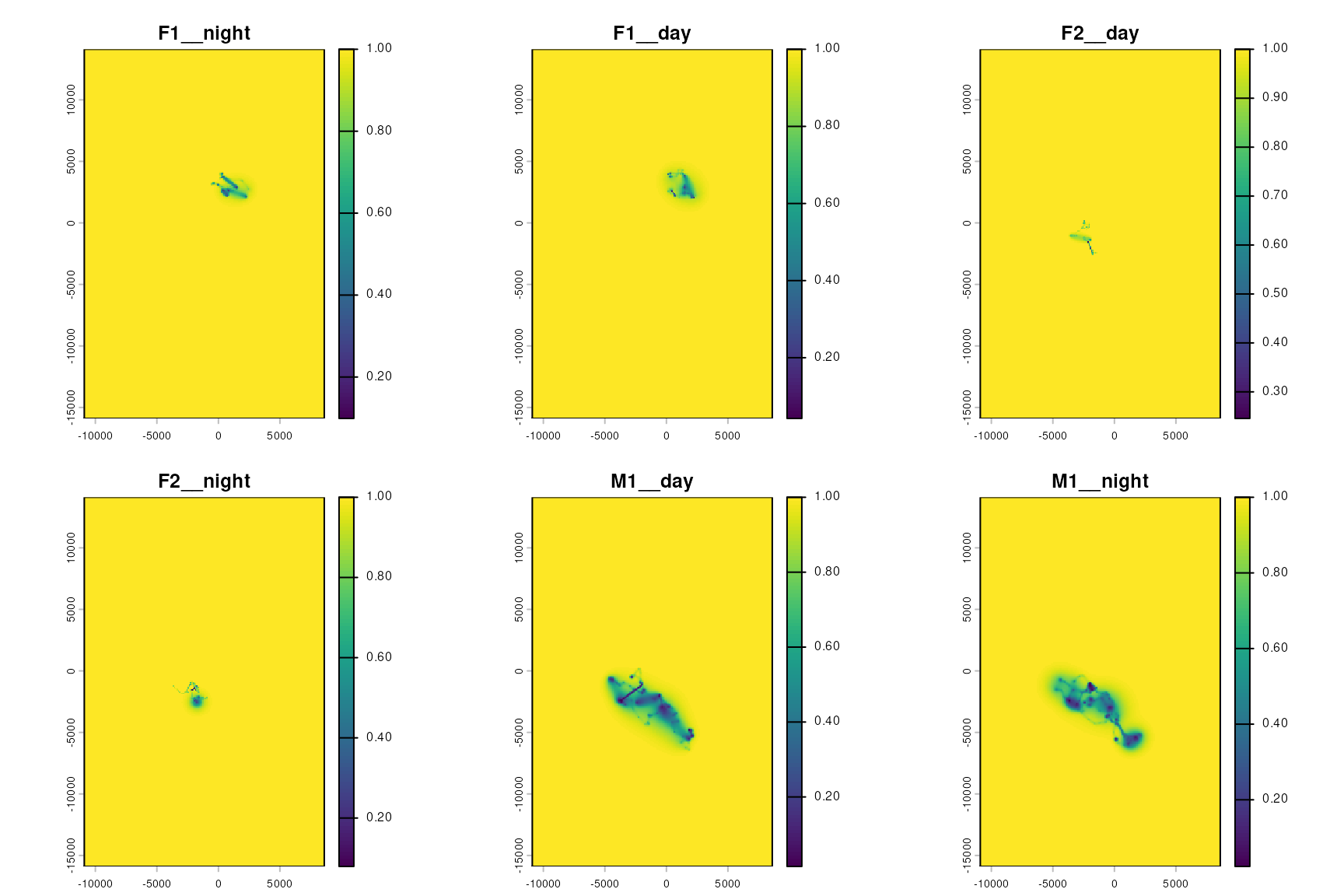

Day / night UDs for F1, F2, M1. Each panel is an Cumulative volume UD on a common grid, so the layers are directly comparable.

Each layer of stk is an ordinary UD with cells summing to 1. To compare “F1 day” against “F1 night” you index the stack with its name: stk[["F1__night"]].

Caveats

Filter out short bursts first. mt_dbbmm_variance() will error or warn on bursts that contain fewer locations than window_size. Compute table(mt_track_id(focal_burst)) and drop sparse contexts before fitting.
Do not burst across long gaps. If day_night flips in the middle of an overnight gap, the burst boundary artificially closes the UD at the two gap endpoints. Mask long-gap segments with mt_mask_segments() after fitting variance, or skip the transition points before labelling. See vignette("UD_gap_aware_ud", package = "move2utils") for the full workflow.
Common-grid discipline. If you compare bursts visually or metrically (e.g. overlap), the multi-track dispatch already puts all layers on the same grid. If you mix outputs from separate dispatches, pass a pre-made SpatRaster to each call.

Idiom B — `split()` and `lapply()`

When each burst needs its own grid, resolution, or parameters, split the object explicitly and iterate.

bursts <- split(focal_p, interaction(mt_track_id(focal_p),
                                       focal_p$day_night,
                                       drop = TRUE))
bursts <- bursts[sapply(bursts, nrow) >= 60]  # drop sparse bursts

var_each <- lapply(bursts, mt_dbbmm_variance,
                    location_error = 25,
                    window_size    = 31,
                    margin         = 11)

## compute each UD on a common grid so they remain stackable
all_xy <- do.call(rbind, lapply(var_each, function(v) {
  data.frame(x = v$track_data$x, y = v$track_data$y)
}))
pts <- sf::st_as_sf(all_xy, coords = c("x", "y"),
                     crs = var_each[[1]]$track_data$crs)
grid <- move2utils:::.make_raster(pts, cell_size = 100, ext = 0.85)

ud_each <- lapply(var_each, mt_dbbmm_ud,
                   location_error = 25, raster = grid, verbose = FALSE)
stk_b <- terra::rast(ud_each)
names(stk_b) <- names(bursts)

This pattern is also what you want when the context implies genuinely different location_error or window_size per burst — for example a tag that switched duty cycle mid-study.

dBGB bursts for directionality contrasts

Everything above works unchanged for mt_dbgb_variance() and mt_dbgb_ud(). dBGB is particularly informative for per-burst contrasts because it separates directed from random space use. Consider a commuting animal where day-time movement is foraging (parallel ≈ perpendicular variance) and night-time is commuting (parallel ≫ perpendicular):

var_list_d <- mt_dbgb_variance(focal_burst, location_error = 25,
                                 window_size = 31, margin = 11)
stk_d <- mt_dbgb_ud(var_list_d, location_error = 25,
                     raster = 100, ext = 0.85)

Contrast the parallel/perpendicular ratios across bursts via mt_motion_variance() on each list element — the ratio is the diagnostic signal that dBGB adds on top of dBBMM.

When a burst should not be a new track

Some contexts are not really bursts at all — they are filters. For instance, to compute a UD only for locations in a specific habitat, the right operation is filter(), not burst(). If the animal never returns to the filtered class, the UD is defined. If it does, you have three options and should choose deliberately:

Compute the UD on the filtered subset only (you get habitat-specific use).
Compute the UD on the whole track and then mask cells outside the habitat of interest.
Compute the UD on the whole track, unmasked, and report the fraction of the UD falling in the habitat.

These answer different questions; the difference is not a detail.

Two idioms

A. Composite track_id

B. split() and iterate