Migratory satellite tracking: Leo the Turkey Vulture

This vignette demonstrates outlier detection on satellite tracking data from a migratory Turkey Vulture (Cathartes aura). The data presents very different challenges from high-frequency GPS data: coarse temporal resolution (~3 fixes/day but highly irregular), large spatial extent (Canada to Venezuela), and extreme variation in step lengths between migratory and stationary phases.

Load data

Leo’s tracking data (2007–2013) is bundled with the package.

library(move2)
library(sf)
library(move2utils)

Leo <- mt_read(system.file("extdata", "Leo-65545.csv.gz",
                           package = "move2utils"))
Leo <- Leo[!st_is_empty(Leo), ]

cat(nrow(Leo), "locations over",
    round(as.numeric(diff(range(mt_time(Leo))), units = "days")),
    "days\n")
#> 35256 locations over 2102 days

## time lag distribution
tl <- as.numeric(diff(mt_time(Leo)), units = "hours")
cat("Time lags: median", round(median(tl), 1), "h,",
    "range", round(min(tl), 1), "--", round(max(tl), 1), "h\n")
#> Time lags: median 1 h, range 1 -- 9253 h

The time lags are extremely variable – from 1 hour to months-long gaps (tag off, overwintering). This makes time normalisation essential.

Why time normalisation matters

Without time normalisation, the method flags long-distance migratory steps as “outliers” because the raw displacement is extreme compared to local foraging movements. With time normalisation, these become moderate speeds – a vulture covering 500 km in 3 days is not unusual.

r_tn <- mt_flag_outliers(Leo, time_normalize = TRUE, plot = FALSE)
#> Calculating movement metrics...
#> ACF-derived alpha: 0.080 (r_speed=0.823, r_angvel=0.008)
#> Calculating probability distributions...
#> Calculating joint probabilities...
#> Identifying outliers...
#> 
#> 3 locations (0.0%) have NA probabilities (includes 7001 stationary fixes) --will be kept.
#> === 31 outliers (0.09% of 35256) ===
r_raw <- mt_flag_outliers(Leo, time_normalize = FALSE, plot = FALSE)
#> Calculating movement metrics...
#> ACF-derived alpha: 0.029 (r_speed=0.108, r_angvel=0.008)
#> Calculating probability distributions...
#> Note: step-length range/IQR = 1780 is extreme;
#>   teleport-class GPS errors are better handled by
#>   mt_filter_gps_quality() (drop fixes with <5 satellites)
#>   and mt_flag_outliers_bridge() (geometric, leverage-immune).
#>   step_transform = "log" is available but can hide
#>   physiologically-plausible joint turn/step outliers.
#> Calculating joint probabilities...
#> Identifying outliers...
#> 
#> 3 locations (0.0%) have NA probabilities (includes 7001 stationary fixes) --will be kept.
#> === 303 outliers (0.86% of 35256) ===

cat("With time normalisation:   ", sum(r_tn$is_outlier), "outliers\n")
#> With time normalisation:    31 outliers
cat("Without time normalisation:", sum(r_raw$is_outlier), "outliers\n")
#> Without time normalisation: 303 outliers

The hundreds of “outliers” without time normalisation are false positives – perfectly normal migratory movements that look extreme only because the raw step length ignores how much time elapsed.

Default detection

result <- mt_flag_outliers(Leo)
#> Calculating movement metrics...
#> ACF-derived alpha: 0.080 (r_speed=0.823, r_angvel=0.008)
#> Calculating probability distributions...
#> Calculating joint probabilities...
#> Identifying outliers...
#> 
#> 3 locations (0.0%) have NA probabilities (includes 7001 stationary fixes) --will be kept.
#> === 31 outliers (0.09% of 35256) ===
#> Creating diagnostic plot...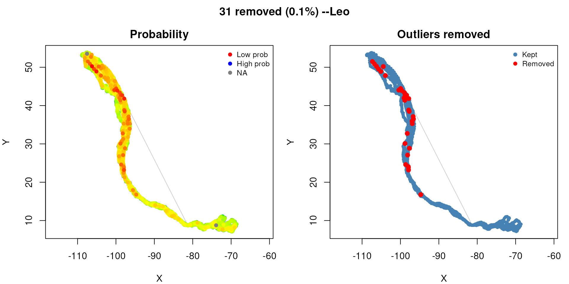

With time normalisation and the default gap-based threshold, Leo’s data shows very few or no outliers. Satellite tracking of a soaring bird produces data that is inherently more variable than GPS tracking of a terrestrial mammal, and the method correctly recognises this as the normal distribution rather than flagging the tails.

Unified detection — `mt_clean_track()`

For routine cleaning, mt_clean_track() composes all four primitives (bridge residual, path-vs-displacement detour ratio, movement-metric probability, step-level speed cap) under a single iterative call, applying the class-aware flag rule by default. Turkey vultures sustain flight speeds around 25 m/s; supplying that as a physiological cap lets the speed primitive peel any spoof- or teleport-class clusters at their boundaries before the other detectors run on the survivors.

clean <- mt_clean_track(Leo, v_max = 25, plot = FALSE)
#> Speed peel (pre-step) at v_max = 25 m/s: 4 fix(es) removed in 1 iteration(s).
#> Iter 1: bridge=13438 prob=11 speed=0 detour=3127 (v_max=25.0) | conjunction=537 | new=537 cumulative=541
#> Iter 2: bridge=10205 prob=41 speed=0 detour=2599 (v_max=25.0) | conjunction=50 | new=50 cumulative=591
#> Iter 3: bridge=10148 prob=21 speed=0 detour=2586 (v_max=25.0) | conjunction=18 | new=18 cumulative=609
#> Iter 4: bridge=10175 prob=23 speed=0 detour=2585 (v_max=25.0) | conjunction=17 | new=17 cumulative=626
#> Iter 5: bridge=10172 prob=23 speed=0 detour=2584 (v_max=25.0) | conjunction=14 | new=14 cumulative=640
#> Iter 6: bridge=10176 prob=16 speed=0 detour=2584 (v_max=25.0) | conjunction=8 | new=8 cumulative=648
#> Iter 7: bridge=10173 prob=25 speed=0 detour=2584 (v_max=25.0) | conjunction=15 | new=15 cumulative=663
#> Iter 8: bridge=10113 prob=23 speed=0 detour=2584 (v_max=25.0) | conjunction=16 | new=16 cumulative=679
#> Iter 9: bridge=10101 prob=22 speed=0 detour=2584 (v_max=25.0) | conjunction=16 | new=16 cumulative=695
#> Iter 10: bridge=10094 prob=26 speed=0 detour=2584 (v_max=25.0) | conjunction=21 | new=21 cumulative=716
#> Iter 11: bridge=10089 prob=37 speed=0 detour=2584 (v_max=25.0) | conjunction=31 | new=31 cumulative=747
#> Iter 12: bridge=10067 prob=25 speed=0 detour=2583 (v_max=25.0) | conjunction=17 | new=17 cumulative=764
#> Iter 13: bridge=10033 prob=39 speed=0 detour=2583 (v_max=25.0) | conjunction=29 | new=29 cumulative=793
#> Iter 14: bridge=10059 prob=32 speed=0 detour=2582 (v_max=25.0) | conjunction=22 | new=22 cumulative=815
#> Iter 15: bridge=10070 prob=18 speed=0 detour=2581 (v_max=25.0) | conjunction=11 | new=11 cumulative=826
#> Iter 16: bridge=10062 prob=3 speed=0 detour=2580 (v_max=25.0) | conjunction=0 | new=0 cumulative=826
#> === mt_clean_track: 826 flagged (2.343% of 35256); stopped: no_new_flags ===
#>     Returning the cleaned track (34430 rows). To inspect what was flagged, re-run with remove = FALSE.
cat("kept", nrow(clean), "of", nrow(Leo), "fixes\n")
#> kept 34430 of 35256 fixes

For long, irregular satellite tracks where you do not have a known physiological cap, the data-driven default (v_max = NULL) is the safe call.

Auto-optimised alpha

For Leo’s irregular data, how much should the auto-difference terms contribute? The auto-optimisation finds out:

r_auto <- mt_flag_outliers(Leo, autodiff_alpha = "auto", plot = FALSE)
#> Calculating movement metrics...
#> Calculating probability distributions...
#> Auto-optimised alpha: 2.0000
#> Calculating joint probabilities...
#> Identifying outliers...
#> 
#> 3 locations (0.0%) have NA probabilities (includes 7001 stationary fixes) --will be kept.
#> === 20 outliers (0.06% of 35256) ===
cat("Outliers with auto-alpha:", sum(r_auto$is_outlier), "\n")
#> Outliers with auto-alpha: 20

Comparison with a regular-sampling track

The contrast with regular, high-frequency sampling is instructive. The bundled CPF_A synthetic track (also used in vignettes 1, 3, 4 and 5) has regular sampling and 23 outliers planted at known positions. On it the detector finds genuine errors that stand out clearly against the otherwise tight distribution:

path <- system.file("extdata/synthetic_tracks.csv.gz",
                    package = "move2utils")
tracks <- mt_read(path)
cpf_a <- filter_track_data(tracks, .track_id = "CPF_A")


r_cpf <- mt_flag_outliers(cpf_a, plot = FALSE)
#> Calculating movement metrics...
#> ACF-derived alpha: 0.215 (r_speed=0.816, r_angvel=0.057)
#> Calculating probability distributions...
#> Note: step-length range/IQR = 8231 is extreme;
#>   teleport-class GPS errors are better handled by
#>   mt_filter_gps_quality() (drop fixes with <5 satellites)
#>   and mt_flag_outliers_bridge() (geometric, leverage-immune).
#>   step_transform = "log" is available but can hide
#>   physiologically-plausible joint turn/step outliers.
#> Calculating joint probabilities...
#> Identifying outliers...
#> 
#> 3 locations (0.2%) have NA probabilities --will be kept.
#> === 11 outliers (0.63% of 1748) ===
cat("CPF_A (regular sampling, 23 planted outliers):",
    sum(r_cpf$is_outlier), "flagged of", nrow(cpf_a), "fixes\n")
#> CPF_A (regular sampling, 23 planted outliers): 11 flagged of 1748 fixes
cat("Leo (vulture, satellite):",
    sum(result$is_outlier), "flagged of", nrow(Leo), "fixes\n")
#> Leo (vulture, satellite): 31 flagged of 35256 fixes

The method adapts to the data: regular high-frequency sampling has a tighter probability distribution where planted errors stand out clearly, while irregular satellite data has wider natural variability that the gap threshold respects.

Multi-scale persistence annotation

The mt_persistence_score() helper takes any flagger’s output and adds a per-flag confidence score: at each of scales = c(2, 4, 8) (the validation scales), it asks whether the flagged fix’s local geometry is still anomalous when viewed over a wider temporal window. Scores range 1 (flagged only at native resolution) to 4 (flagged at every validation scale). The helper does not modify is_outlier – it only annotates.

annotated <- mt_persistence_score(result, silent = TRUE)
flagged <- which(annotated$is_outlier)
cat("Persistence score distribution among flagged fixes:\n")
#> Persistence score distribution among flagged fixes:
print(table(annotated$persistence_count[flagged]))
#> 
#>  4 
#> 31

See vignette("OUTLIER_5_persistence_score", package = "move2utils") for the empirical class-conditional discrimination analysis on synthetic CPF data.