Directional UDs with the dynamic bivariate Gaussian bridge (dBGB)

When an animal travels in a committed direction — a migration leg, a daily commute between roost and foraging site — you intuitively expect its utilisation distribution to be elongated along that direction, not a round blob. The standard dynamic Brownian bridge (dBBMM) doesn’t capture this: it treats movement between two fixes as wandering equally in all directions, so it spreads the UD into a circle around each step. For a directed traveller, that over-spreads sideways and under-represents the actual route.

The dynamic bivariate Gaussian bridge (dBGB) fixes this. It splits the bridge between two fixes into two parts: one along the direction of travel and one perpendicular to it. Each part has its own variance. When the animal is moving fast and straight, the along-track variance is large (it could be anywhere on the line) but the across-track variance is small (it’s not off to one side). The resulting UD hugs the travel axis instead of spreading into a disc.

mt_dbgb_variance() and mt_dbgb_ud() are the directional counterparts to mt_dbbmm_variance() and mt_dbbmm_ud(). They share the same two-step workflow (fit the variance, then rasterise the UD) and return UDs on the same kind of terra grid, so you can swap them in without restructuring downstream code. If you used move::brownian.bridge.dyn() before, the dBGB is the directional generalisation: when the parallel and perpendicular variances are equal, dBGB collapses back to dBBMM.

When to reach for dBGB rather than dBBMM

Movement mode	Reach for
Foraging, resting, random area use	`mt_dbbmm_*` (isotropy is a fine prior)
Commuting, migration legs, directed travel	`mt_dbgb_*`
Mixed (the usual case)	Either. dBGB generalises dBBMM: when parallel and perpendicular variances are equal, the two agree. It is safe to default to dBGB if you suspect directionality matters.

The cost is modest — roughly twice the compute of dBBMM because two variances have to be estimated per window — and the benefit is a UD that respects the direction of travel.

Load and project

library(move2)
library(sf)
library(dplyr)
library(terra)
library(move2utils)

fishers <- mt_read(mt_example())
fishers <- fishers[!st_is_empty(fishers), ]

## Leroy again, first 500 fixes for a fast build
leroy <- filter_track_data(fishers, .track_id = "M1")
leroy <- slice(leroy,1:500)
leroy_p <- st_transform(leroy, mt_aeqd_crs(leroy))

Fit a dBGB

The signature mirrors dBBMM. mt_dbgb_variance() returns an S3 object holding the parallel and perpendicular standard deviations; mt_motion_variance() extracts them as a data.frame with columns para and orth.

var_dbgb <- mt_dbgb_variance(
  leroy_p,
  location_error = 20,
  window_size    = 31,
  margin         = 11
)

## per-location directional variances
v_df <- mt_motion_variance(var_dbgb)
summary(v_df)
#>       para             orth        
#>  Min.   :   0.0   Min.   :   0.00  
#>  1st Qu.: 211.1   1st Qu.:  45.92  
#>  Median :2665.5   Median : 611.22  
#>  Mean   :2272.7   Mean   :1427.74  
#>  3rd Qu.:3500.0   3rd Qu.:2292.49  
#>  Max.   :9634.7   Max.   :7443.30  
#>  NAs    :21       NAs    :21

A quick comparison of the two dimensions over time tells you whether the animal is directional. The ratio para / orth > 1 indicates elongation along the direction of travel.

time_days <- as.numeric(mt_time(leroy_p) - mt_time(leroy_p)[1], units = "days")
plot(time_days, v_df$para, type = "l", col = "steelblue", lwd = 1.5,
     ylim = c(0, max(v_df, na.rm = TRUE)),
     xlab = "time (days since start)", ylab = "variance (m^2)",
     main = "parallel vs perpendicular variance")
lines(time_days, v_df$orth, col = "firebrick", lwd = 1.5)
legend("topright", c("parallel", "perpendicular"),
       col = c("steelblue", "firebrick"), lwd = 1.5, bty = "n")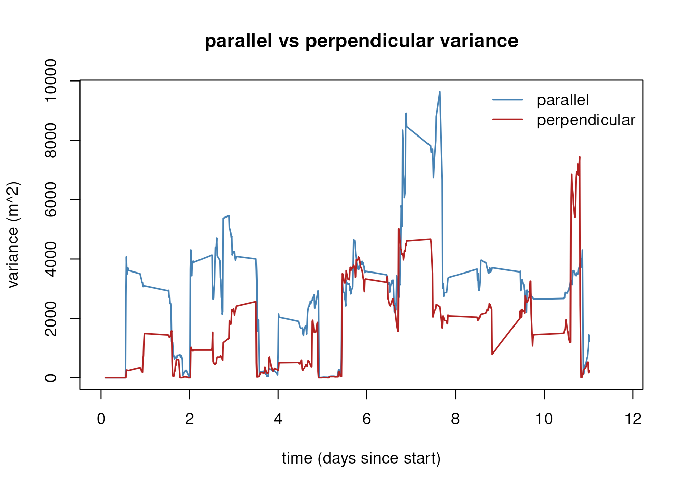

Rasterise the UD

mt_dbgb_ud() accepts the variance object (or a move2 track directly, in which case it estimates variance internally) and produces a SpatRaster whose cells sum to 1.

ud_dbgb <- mt_dbgb_ud(var_dbgb, location_error = 20,
                       raster = 100, ext = 0.85)

terra::plot(ud_dbgb, main = "dBGB utilisation distribution")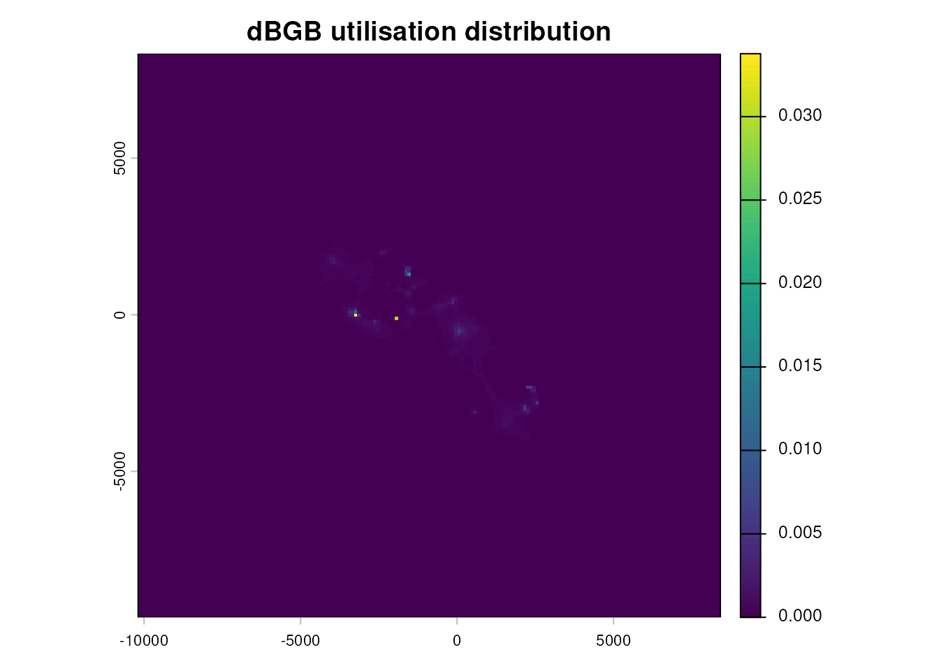

If you see The raster does not extent far enough ..., increase ext (padding around the auto-generated raster) or pass a pre-made SpatRaster that is large enough. The dBGB kernel needs more margin than dBBMM when the parallel variance is high, because the bridge extends further along the direction of travel.

Cumulative-volume UD and isopleths

ud_volume() converts the probability-density UD into cumulative- volume space and works on any UD SpatRaster, dBBMM or dBGB (see vignette("UD_dbbmm_ud", package = "move2utils") for more details).

vud_dbgb <- ud_volume(ud_dbgb)
terra::plot(vud_dbgb, main = "dBGB cumulative volume")
terra::contour(vud_dbgb, levels = c(0.5, 0.95), add = TRUE,
               lty = c(2, 1), lwd = c(0.5, 0.5))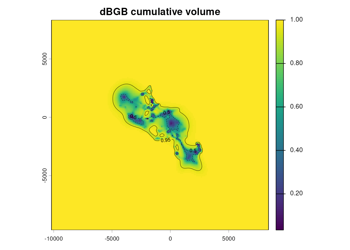

Side-by-side: dBBMM vs dBGB on the same track

A two-panel comparison reveals where the two models differ. Same track, same grid, same location_error:

var_dbbmm <- mt_dbbmm_variance(
  leroy_p, location_error = 20,
  window_size = 31, margin = 11
)
ud_dbbmm <- mt_dbbmm_ud(var_dbbmm, location_error = 20, raster = 100,
                         ext = 0.85, verbose = FALSE)

## put both UDs on the same extent so the two panels are comparable
common_ext <- terra::union(terra::ext(ud_dbbmm), terra::ext(ud_dbgb))
ud_dbbmm <- terra::extend(ud_dbbmm, common_ext)
ud_dbgb  <- terra::extend(ud_dbgb,  common_ext)

## plotting the cumulative-volume UD for better visualization
vud_dbbmm <- ud_volume(ud_dbbmm)
vud_dbgb <- ud_volume(ud_dbgb)
par(mfrow = c(1, 2))
terra::plot(vud_dbbmm, main = "dBBMM (isotropic)")
terra::plot(vud_dbgb,  main = "dBGB (directional)")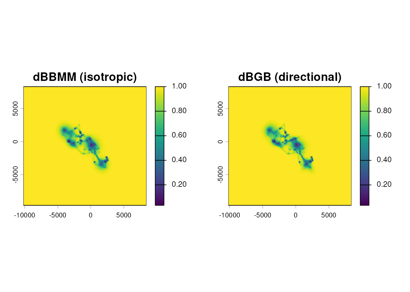

On a fisher, which foraged extensively over this window, the two UDs will look similar. On a commuting or migrating animal, the dBGB UD narrows visibly along the travel legs. Try the Leo turkey vulture example (vignette("OUTLIER_example_leo_migration", package = "move2utils")) for a clearer case.

Gap handling

dBGB exposes a segment-level interest flag (seg_interest) rather than a location-level interest flag. The semantics are the same — a segment marked FALSE is skipped during UD integration — but you index it one shorter than the track length (n-1 segments).

lag_min <- as.numeric(mt_time_lags(leroy_p, units = "min"))
var_dbgb$seg_interest[lag_min > 300] <- FALSE

ud_masked <- mt_dbgb_ud(var_dbgb, location_error = 20, raster = 100,
                         ext = 0.85, verbose = FALSE)